Adaptive Large Neighborhood Search Enhances Global Protein-Protein Network Alignment

VNU Journal of Science: Comp. Science & Com. Eng., Vol. 35, No. 1 (2019) 46-55 
46 
Original Article 
Adaptive Large Neighborhood Search Enhances Global 
Protein-Protein Network Alignment 
Vu Thi Ngoc Anh1, 2, Nguyen Trong Dong2, 
Nguyen Vu Hoang Vuong2, Dang Thanh Hai3, *, Do Duc Dong3, * 
1
The Hanoi college of Industrial Economics, 
2VNU University of Engineering and Technology, 144 Xuan Thuy, Cau Giay, Hanoi, Vietnam, 
3Bingo Biomedical Informatics Laboratory (Bingo Lab), Faculty of Information Technology, VNU 
University of Engineering and Technology 
Received 05 March 2018 
Revised 19 May 2019; Accepted 27 May 2019 
Abstract: Aligning protein-protein interaction networks from different species is a useful 
mechanism for figuring out orthologous proteins, predicting/verifying protein unknown functions 
or constructing evolutionary relationships. The network alignment problem is proved to be 
NP-hard, requiring exponential-time algorithms, which is not feasible for the fast growth of 
biological data. In this paper, we present a novel global protein-protein interaction network 
alignment algorithm, which is enhanced with an extended large neighborhood search heuristics. 
Evaluated on benchmark datasets of yeast, fly, human and worm, the proposed algorithm 
outperforms state-of-the-art algorithms. Furthermore, the complexity of ours is polynomial, thus 
being scalable to large biological networks in practice. 
Keywords: Heuristic, Protein-protein interaction networks, network alignment, neighborhood search. 
1. Introduction* 
Advanced high-throughput biotechnologies 
have been revealing numerous interactions 
between proteins at large-scales, for various 
species. Analyzing those networks is, thus, 
becoming emerged, such as network topology 
analyses [1], network module detection [2], 
evolutionary network pattern discovery [3] and 
network alignment [4], etc. 
________ 
* Corresponding author. 
 E-mail address: {hai.dang, dongdoduc}@vnu.edu.vn 
 https://doi.org/10.25073/2588-1086/vnucsce.228 
From biological perspectives, a good 
alignment between protein-protein networks 
(PPI) in different species could provide a strong 
evidence for (i) predicting unknown functions 
of orthologous proteins in a less-well studied 
species, or (ii) verifying those with known 
functions [5], or (iii) detecting common 
orthologous pathways between species [6] or 
(iv) reconstructing the evolutionary dynamics 
of various species [4]. 
PPI network alignment methods fall into two 
categories: local alignment and global alignment. 
The former aims identifying 
sub-networks that are conserved across networks 
in terms of topology and/or sequence similarity 
V.T.N. Anh et al. / VNU Journal of Science: Comp. Science & Com. Eng., Vol. 35, No. 1 (2019) 46-55 47 
[7-11]. Sub-networks within a single PPI network 
are very often returned as parts of local alignment, 
giving rise to ambiguity, as a protein may be 
matched with many proteins from another target 
network [12]. The latter, on the other hand, aims 
to align the whole networks, providing 
unambiguous one-to-one mappings between 
proteins of different networks [4, 12, 13-16]. 
The major challenging of network 
alignment is computational complexity. It 
becomes even more apparent as PPI networks 
are becoming larger (Network may be of up to 
104 or even 105 interactions). Nevertheless, 
existing approaches are optimized only for 
either the performance accuracy or the 
run-time, but not for both as expected, for 
networks of medium sizes. In this paper, we 
introduce a new global PPI network (GPN) 
algorithms that exploit the adaptive large 
neighborhood search. Thorough experimental 
results indicate that our proposed algorithm 
could attain better performance of high 
accuracy in polynomial run-time when 
compared to other state-of-the-art algorithms. 
2. Problem statement 
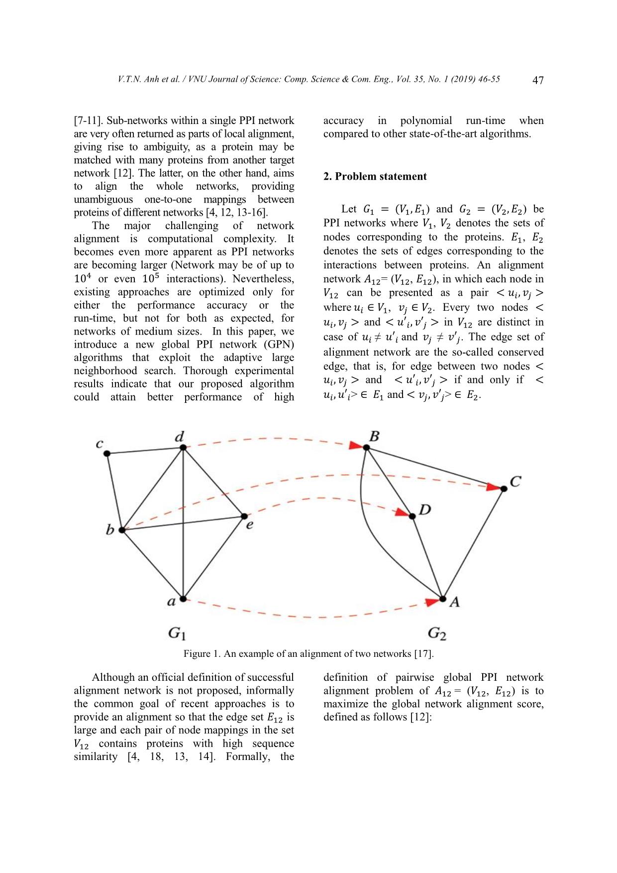
Let 𝐺1 = (𝑉1, 𝐸1) and 𝐺2 = (𝑉2, 𝐸2) be 
PPI networks where 𝑉1, 𝑉2 denotes the sets of 
nodes corresponding to the proteins. 𝐸1, 𝐸2 
denotes the sets of edges corresponding to the 
interactions between proteins. An alignment 
network 𝐴12= (𝑉12, 𝐸12), in which each node in 
𝑉12 can be presented as a pair 
where 𝑢𝑖 ∈ 𝑉1, 𝑣𝑗 ∈ 𝑉2. Every two nodes <
𝑢𝑖, 𝑣𝑗 > and in 𝑉12 are distinct in 
case of 𝑢𝑖 ≠ 𝑢′𝑖 and 𝑣𝑗 ≠ 𝑣′𝑗. The edge set of 
alignment network are the so-called conserved 
edge, that is, for edge between two nodes <
𝑢𝑖, 𝑣𝑗 > and if and only if <
𝑢𝑖, 𝑢′𝑖> ∈ 𝐸1 and ∈ 𝐸2. 
Figure 1. An example of an alignment of two networks [17]. 
Although an official definition of successful 
alignment network is not proposed, informally 
the common goal of recent approaches is to 
provide an alignment so that the edge set 𝐸12 is 
large and each pair of node mappings in the set 
𝑉12 contains proteins with high sequence 
similarity [4, 18, 13, 14]. Formally, the 
definition of pairwise global PPI network 
alignment problem of 𝐴12 = (𝑉12, 𝐸12) is to 
maximize the global network alignment score, 
defined as follows [12]: 
V.T.N. Anh et al. / VNU Journal of Science: Comp. Science & Com. Eng., Vol. 35, No. 1 (2019) 46-55 
48 
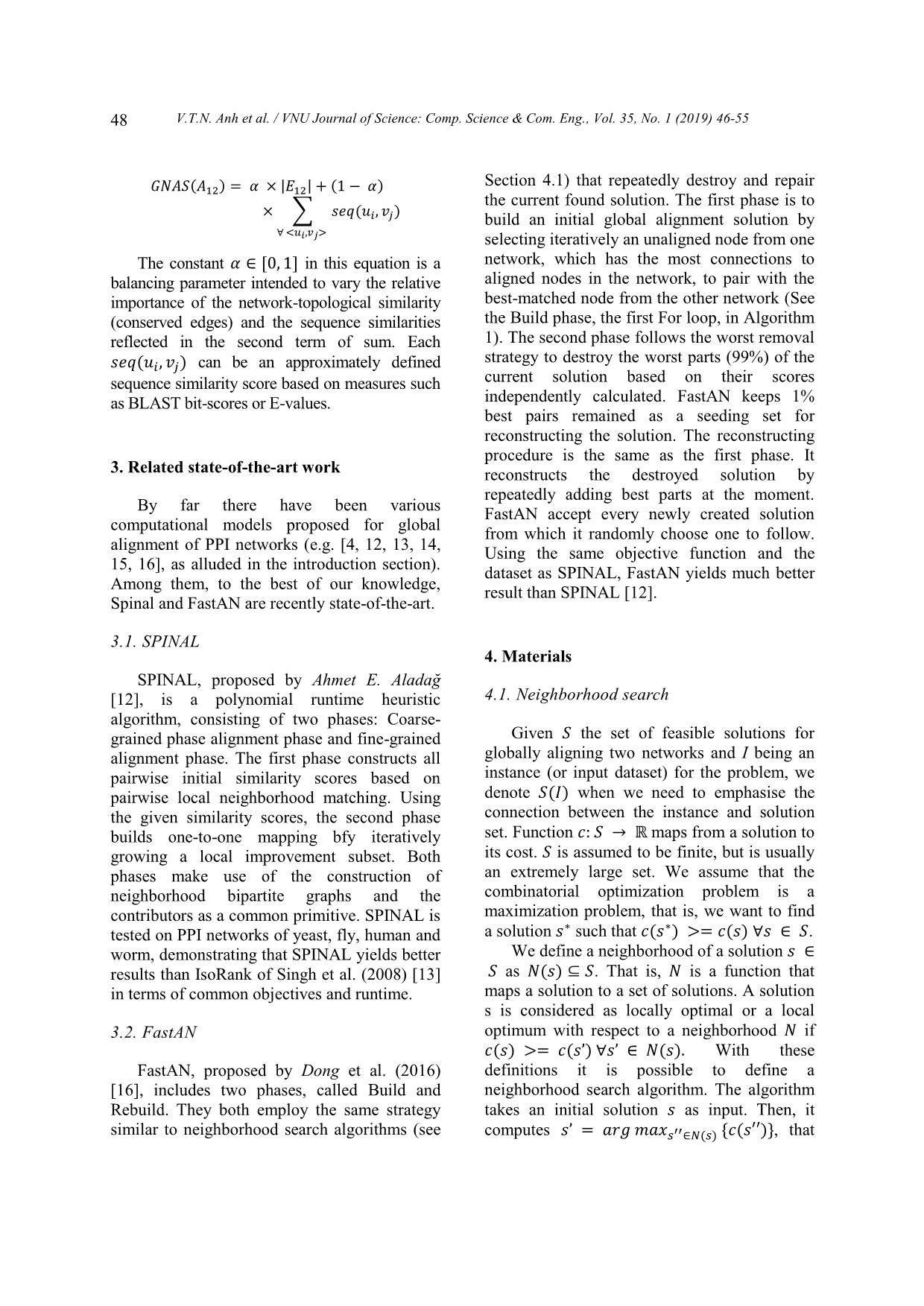
𝐺𝑁𝐴𝑆(𝐴12) = 𝛼 × |𝐸12| + (1 − 𝛼)
× ∑ 𝑠𝑒𝑞(𝑢𝑖, 𝑣𝑗)
∀ 
The constant 𝛼 ∈ [0, 1] in this equation is a 
balancing parameter intended to vary the relative 
importance of the network-topological similarity 
(conserved edges) and the sequence similarities 
reflected in the second term of sum. Each 
𝑠𝑒𝑞(𝑢𝑖, 𝑣𝑗) can be an approximately defined 
sequence similarity score based on measures such 
as BLAST bit-scores or E-values. 
3. Related state-of-the-art work 
By far there have been various 
computational models proposed for global 
alignment of PPI networks (e.g. [4, 12, 13, 14, 
15, 16], as alluded in the introduction section). 
Among them, to the best of our knowledge, 
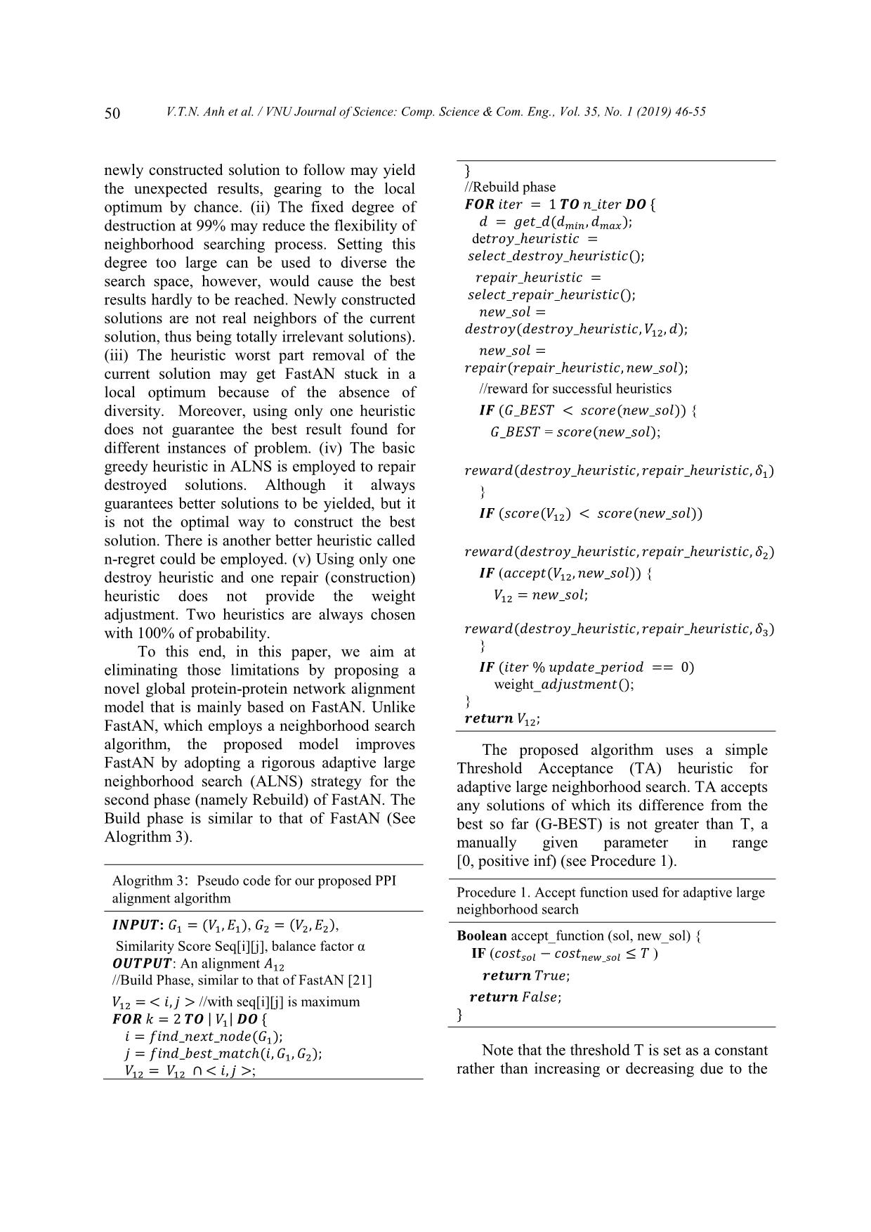
Spinal and  ... is 
elegans 
2805 4495 
Homo sapiens 9633 34327 
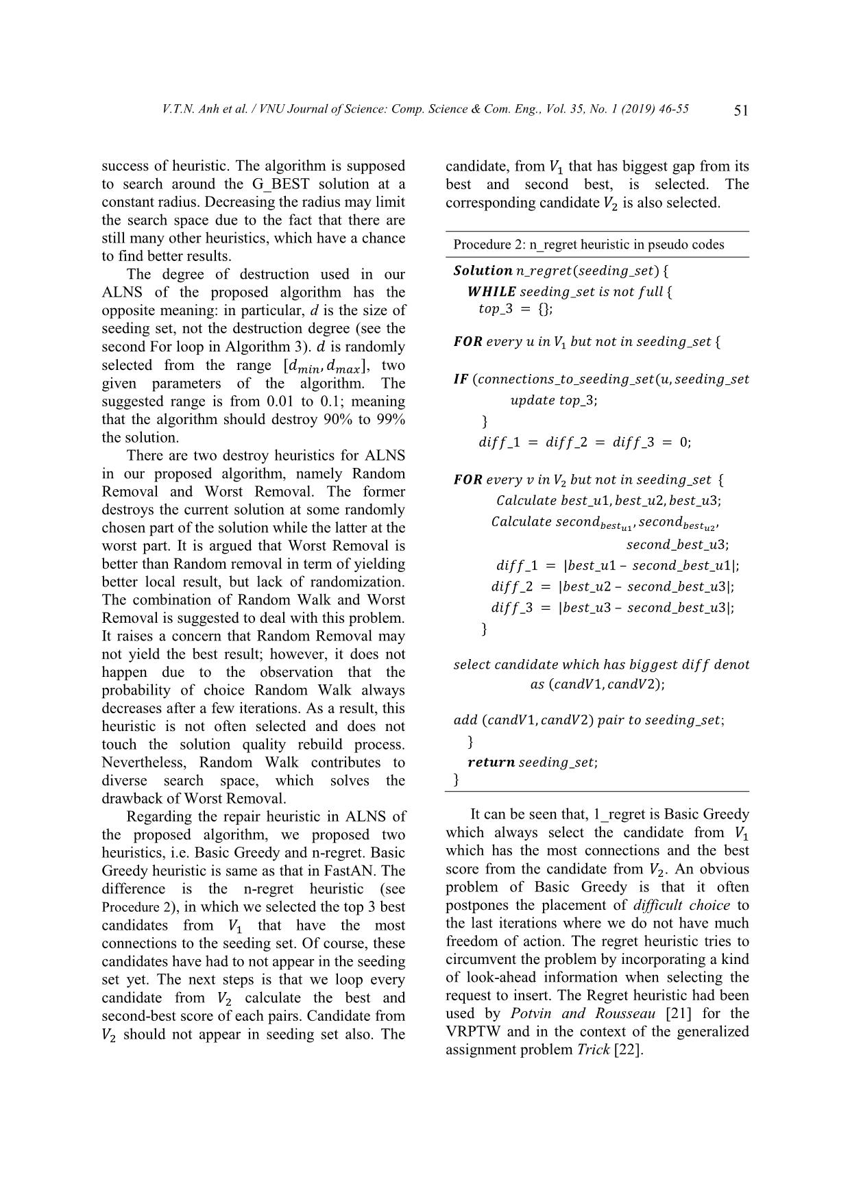
6.2. Experimental results in comparison 
with FastAN 
We first examine the efficiency of each 
improvement in the proposed algorithm 
including strategy of choosing a degree of 
destruction, different destroy and repair 
functions. The objective function is described in 
section 1.2. Results for each improvement are 
compared with those of FastAN. 
6.3. Improvement with randomization of 
destruction degree 
Here is the first improvement, we keep all 
settings as same as the original FastAN 
algorithm except for only the strategy of 
choosing 𝑑. FastAN is using destroy heuristic 
Worst Removal, and repair heuristic is Basic 
Greedy. It fixed 𝑑 = 99%, while we randomize 
parameter 𝑑 in range [𝑑𝑚𝑖𝑛, 𝑑𝑚𝑎𝑥]. 
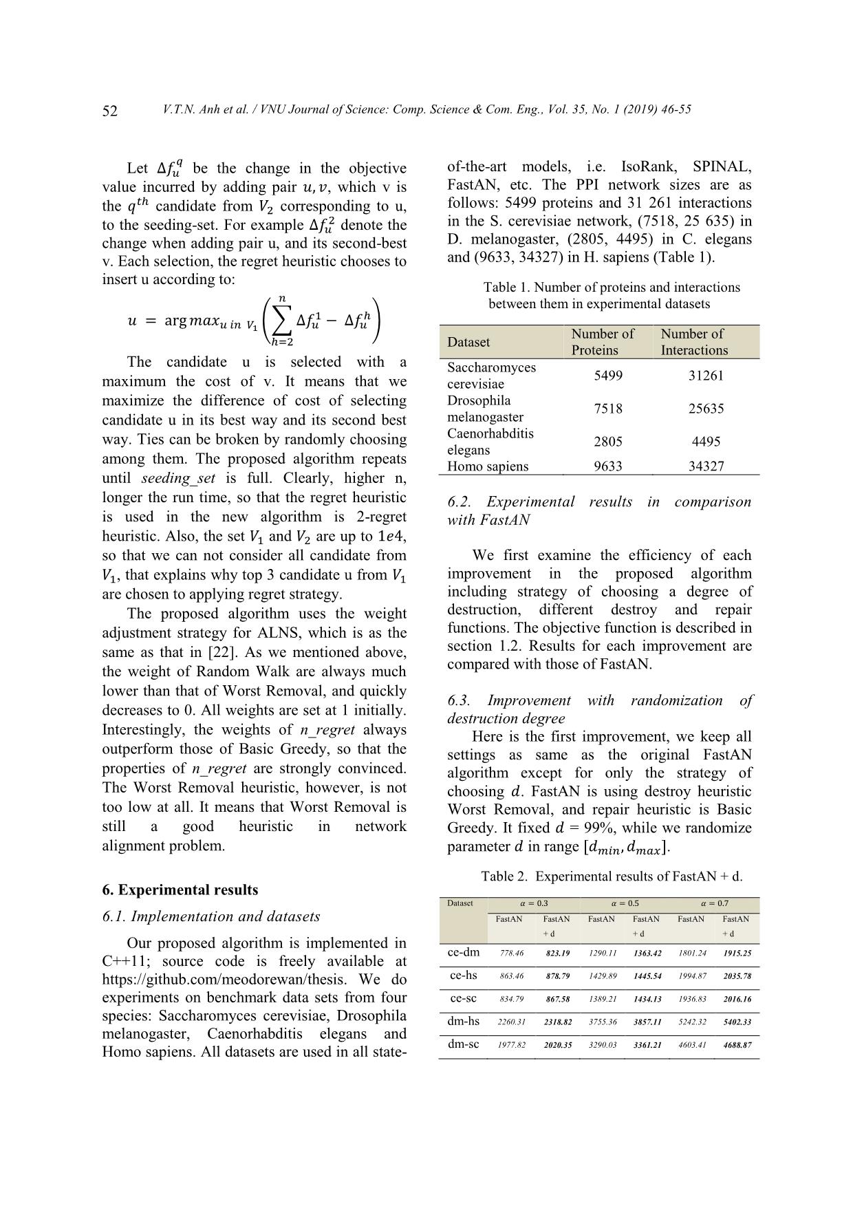
Table 2. Experimental results of FastAN + d. 
Dataset 𝛼 = 0.3 𝛼 = 0.5 𝛼 = 0.7 
FastAN FastAN 
+ d 
FastAN FastAN 
+ d 
FastAN FastAN 
+ d 
ce-dm 778.46 823.19 1290.11 1363.42 1801.24 1915.25 
ce-hs 863.46 878.79 1429.89 1445.54 1994.87 2035.78 
ce-sc 834.79 867.58 1389.21 1434.13 1936.83 2016.16 
dm-hs 2260.31 2318.82 3755.36 3857.11 5242.32 5402.33 
dm-sc 1977.82 2020.35 3290.03 3361.21 4603.41 4688.87 
V.T.N. Anh et al. / VNU Journal of Science: Comp. Science & Com. Eng., Vol. 35, No. 1 (2019) 46-55 53 
hs-sc 2268.21 2342.29 3772.96 3911.03 5279.88 5444.05 
Through the experimental results shown in 
Table 2, we can conclude that the strategy of 
choosing destruction degree is advantaged. The 
results are much better than that of original 
FastAN with fixed 𝑑 at 99%. The reason is that 
fixed parameter 𝑑 may limit the search space 
and be difficult to find a new local optimum. 
By randomizing 𝑑 in range [𝑑𝑚𝑖𝑛, 𝑑𝑚𝑎𝑥], we 
can diverse the neighborhoods and be able to 
find better optimum. 
6.4. Improvement with destroy heuristic 
Random Removal 
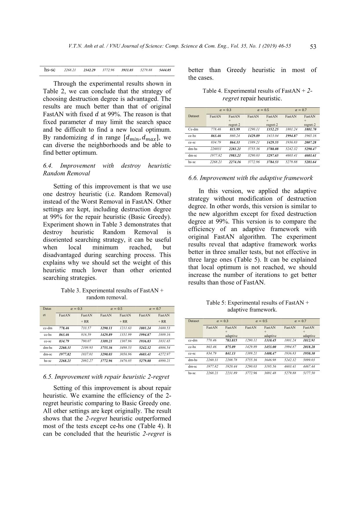
Setting of this improvement is that we use 
one destroy heuristic (i.e. Random Removal) 
instead of the Worst Removal in FastAN. Other 
settings are kept, including destruction degree 
at 99% for the repair heuristic (Basic Greedy). 
Experiment shown in Table 3 demonstrates that 
destroy heuristic Random Removal is 
disoriented searching strategy, it can be useful 
when local minimum reached, but 
disadvantaged during searching process. This 
explains why we should set the weight of this 
heuristic much lower than other oriented 
searching strategies. 
Table 3. Experimental results of FastAN + 
random removal. 
Datas
et 
𝛼 = 0.3 𝛼 = 0.5 𝛼 = 0.7 
FastAN FastAN 
+ RR 
FastAN FastAN 
+ RR 
FastAN FastAN 
+ RR 
ce-dm 778.46 733.57 1290.11 1211.63 1801.24 1680.53 
ce-hs 863.46 816.59 1429.89 1351.99 1994.87 1889.16 
ce-sc 834.79 790.07 1389.21 1307.96 1936.83 1831.65 
dm-hs 2260.31 2109.93 3755.36 3498.53 5242.32 4886.54 
dm-sc 1977.82 1837.01 3290.03 3056.96 4603.41 4272.97 
hs-sc 2268.21 2092.27 3772.96 3476.05 5279.88 4890.21 
6.5. Improvement with repair heuristic 2-regret 
Setting of this improvement is about repair 
heuristic. We examine the efficiency of the 2-
regret heuristic comparing to Basic Greedy one. 
All other settings are kept originally. The result 
shows that the 2-regret heuristic outperformed 
most of the tests except ce-hs one (Table 4). It 
can be concluded that the heuristic 2-regret is 
better than Greedy heuristic in most of 
the cases. 
Table 4. Experimental results of FastAN + 2-
regret repair heuristic. 
Dataset 
𝛼 = 0.3 𝛼 = 0.5 𝛼 = 0.7 
FastAN FastAN 
+ 
regret-2 
FastAN FastAN 
+ 
regret-2 
FastAN FastAN 
+ 
regret-2 
Ce-dm 778.46 815.99 1290.11 1352.25 1801.24 1881.70 
ce-hs 863.46 860.24 1429.89 1413.04 1994.87 1965.16 
ce-sc 834.79 864.33 1389.21 1429.55 1936.83 2007.28 
dm-hs 226031 2281.21 3755.36 3788.08 5242.32 5290.47 
dm-sc 1977.82 1983.21 3290.03 3297.65 4603.41 4603.61 
hs-sc 2268.21 2274.16 3772.96 3784.53 5279.88 5283.64 
6.6. Improvement with the adaptive framework 
In this version, we applied the adaptive 
strategy without modification of destruction 
degree. In other words, this version is similar to 
the new algorithm except for fixed destruction 
degree at 99%. This version is to compare the 
efficiency of an adaptive framework with 
original FastAN algorithm. The experiment 
results reveal that adaptive framework works 
better in three smaller tests, but not effective in 
three large ones (Table 5). It can be explained 
that local optimum is not reached, we should 
increase the number of iterations to get better 
results than those of FastAN. 
Table 5: Experimental results of FastAN + 
adaptive framework. 
Dataset 𝛼 = 0.3 𝛼 = 0.5 𝛼 = 0.7 
FastAN FastAN 
+ 
adaptive 
FastAN FastAN 
+ 
adaptive 
FastAN FastAN 
+ 
adaptive 
ce-dm 778.46 783.815 1290.11 1310.45 1801.24 1812.91 
ce-hs 863.46 875.09 1429.89 1453.00 1994.87 2018.28 
ce-sc 834.79 841.13 1389.21 1408.47 1936.83 1950.30 
dm-hs 2260.31 2208.78 3755.36 3646.98 5242.32 5099.03 
dm-sc 1977.82 1920.44 3290.03 3195.56 4603.41 4467.44 
hs-sc 2268.21 2231.89 3772.96 3691.48 5279.88 5177.50 
V.T.N. Anh et al. / VNU Journal of Science: Comp. Science & Com. Eng., Vol. 35, No. 1 (2019) 46-55 
54 
Table 6. Parameters settings of the proposed 
algorithm 
Parameter Describe Setting 
𝑑𝑚𝑖𝑛 The lower bound of degree of 
destruction 
0.01 
𝑑𝑚𝑎𝑥 The upper bound of degee of 
destruction 
0.1 
N_RUN The number of iteration 100 
PERIOD The update period for weight 
adjustment 
5 
ρ The degenerative factor 0.1 
𝛿1 Reward for solution which 
has best cost so far 
0.8 
𝛿2 Reward for solution which 
has better cost 
0.3 
𝛿3 Reward for solution which is 
accepted 
0 
N_TEST Number of execution to test 
the stability of algorithm 
10 
T Threshold 5 
6.7. Results in terms of alignment objectives 
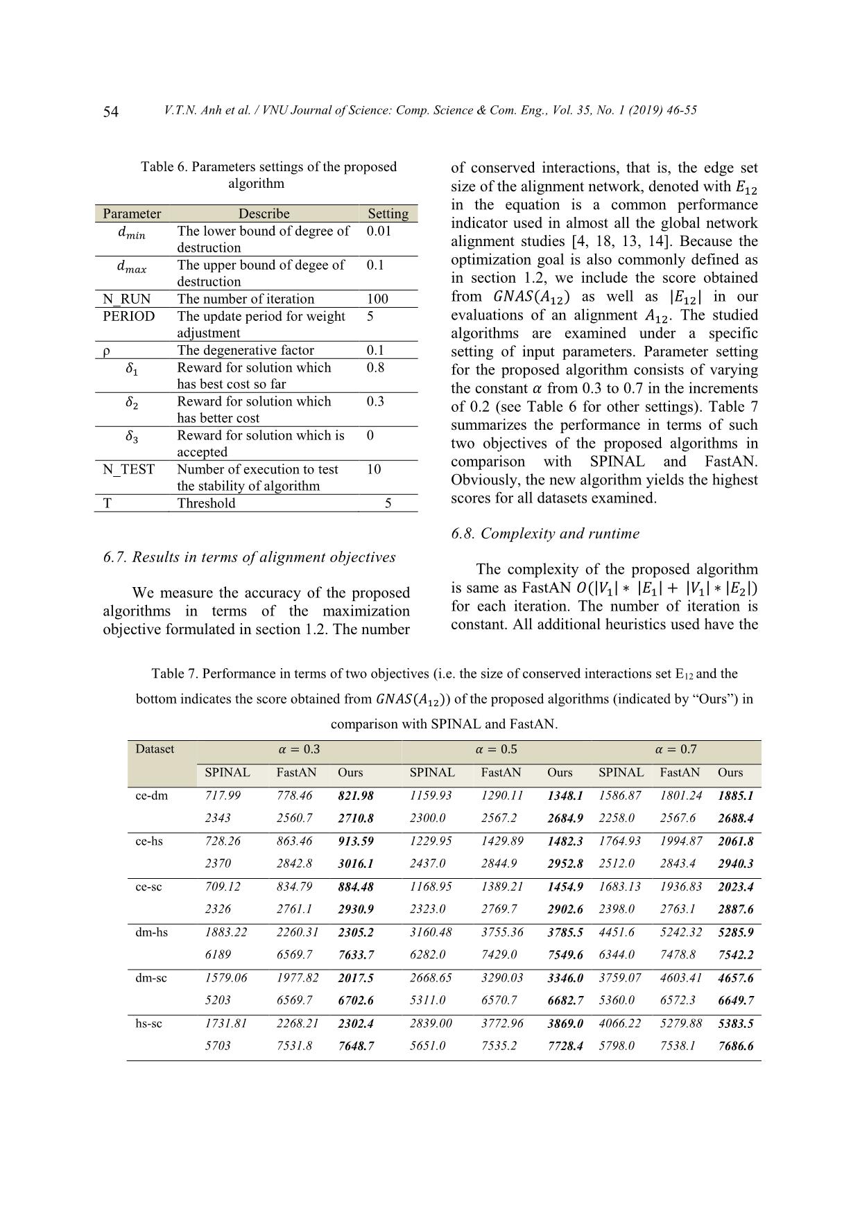
 We measure the accuracy of the proposed 
algorithms in terms of the maximization 
objective formulated in section 1.2. The number 
of conserved interactions, that is, the edge set 
size of the alignment network, denoted with 𝐸12 
in the equation is a common performance 
indicator used in almost all the global network 
alignment studies [4, 18, 13, 14]. Because the 
optimization goal is also commonly defined as 
in section 1.2, we include the score obtained 
from 𝐺𝑁𝐴𝑆(𝐴12) as well as |𝐸12| in our 
evaluations of an alignment 𝐴12. The studied 
algorithms are examined under a specific 
setting of input parameters. Parameter setting 
for the proposed algorithm consists of varying 
the constant 𝛼 from 0.3 to 0.7 in the increments 
of 0.2 (see Table 6 for other settings). Table 7 
summarizes the performance in terms of such 
two objectives of the proposed algorithms in 
comparison with SPINAL and FastAN. 
Obviously, the new algorithm yields the highest 
scores for all datasets examined. 
6.8. Complexity and runtime 
The complexity of the proposed algorithm 
is same as FastAN 𝑂(|𝑉1| ∗ |𝐸1| + |𝑉1| ∗ |𝐸2|) 
for each iteration. The number of iteration is 
constant. All additional heuristics used have the 
Table 7. Performance in terms of two objectives (i.e. the size of conserved interactions set E12 and the 
bottom indicates the score obtained from 𝐺𝑁𝐴𝑆(𝐴12)) of the proposed algorithms (indicated by “Ours”) in 
comparison with SPINAL and FastAN. 
Dataset 𝛼 = 0.3 𝛼 = 0.5 𝛼 = 0.7 
SPINAL FastAN Ours SPINAL FastAN Ours SPINAL FastAN Ours 
ce-dm 717.99 
2343 
778.46 
2560.7 
821.98 
2710.8 
1159.93 
2300.0 
1290.11 
2567.2 
1348.1 
2684.9 
1586.87 
2258.0 
1801.24 
2567.6 
1885.1 
2688.4 
ce-hs 728.26 
2370 
863.46 
2842.8 
913.59 
3016.1 
1229.95 
2437.0 
1429.89 
2844.9 
1482.3 
2952.8 
1764.93 
2512.0 
1994.87 
2843.4 
2061.8 
2940.3 
ce-sc 709.12 
2326 
834.79 
2761.1 
884.48 
2930.9 
1168.95 
2323.0 
1389.21 
2769.7 
1454.9 
2902.6 
1683.13 
2398.0 
1936.83 
2763.1 
2023.4 
2887.6 
dm-hs 1883.22 
6189 
2260.31 
6569.7 
2305.2 
7633.7 
3160.48 
6282.0 
3755.36 
7429.0 
3785.5 
7549.6 
4451.6 
6344.0 
5242.32 
7478.8 
5285.9 
7542.2 
dm-sc 1579.06 
5203 
1977.82 
6569.7 
2017.5 
6702.6 
2668.65 
5311.0 
3290.03 
6570.7 
3346.0 
6682.7 
3759.07 
5360.0 
4603.41 
6572.3 
4657.6 
6649.7 
hs-sc 1731.81 
5703 
2268.21 
7531.8 
2302.4 
7648.7 
2839.00 
5651.0 
3772.96 
7535.2 
3869.0 
7728.4 
4066.22 
5798.0 
5279.88 
7538.1 
5383.5 
7686.6 
V.T.N. Anh et al. / VNU Journal of Science: Comp. Science & Com. Eng., Vol. 35, No. 1 (2019) 46-55 55 
same complexity as it is in Rebuild phase. The 
proposed algorithm’s runtime is also same as 
FastAN’s runtime. 
The hardware used to run the experiment is 
an Intel(R) Xeon(R) CPU E5-2697 v4 @ 
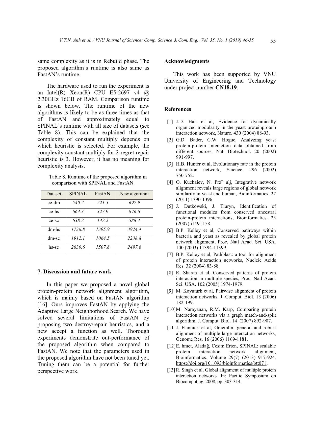
2.30GHz 16GB of RAM. Comparison runtime 
is shown below. The runtime of the new 
algorithms is likely to be as three times as that 
of FastAN and approximately equal to 
SPINAL’s runtime with all size of datasets (see 
Table 8). This can be explained that the 
complexity of constant multiply depends on 
which heuristic is selected. For example, the 
complexity constant multiply for 2-regret repair 
heuristic is 3. However, it has no meaning for 
complexity analysis. 
Table 8. Runtime of the proposed algorithm in 
comparison with SPINAL and FastAN. 
Dataset SPINAL FastAN New algorithm 
ce-dm 540.2 221.5 697.9 
ce-hs 664.3 327.9 846.6 
ce-sc 638.2 142.2 588.4 
dm-hs 1736.8 1395.9 3924.4 
dm-sc 1912.1 1064.5 2238.8 
hs-sc 2630.6 1507.8 2497.6 
7. Discussion and future work 
In this paper we proposed a novel global 
protein-protein network alignment algorithm, 
which is mainly based on FastAN algorithm 
[16]. Ours improves FastAN by applying the 
Adaptive Large Neighborhood Search. We have 
solved several limitations of FastAN by 
proposing two destroy/repair heuristics, and a 
new accept a function as well. Thorough 
experiments demonstrate out-performance of 
the proposed algorithm when compared to 
FastAN. We note that the parameters used in 
the proposed algorithm have not been tuned yet. 
Tuning them can be a potential for further 
perspective work. 
Acknowledgments 
This work has been supported by VNU 
University of Engineering and Technology 
under project number CN18.19. 
References 
[1] J.D. Han et al, Evidence for dynamically 
organized modularity in the yeast proteinprotein 
interaction network, Nature. 430 (2004) 88-93. 
[2] G.D. Bader, C.W. Hogue, Analyzing yeast 
protein-protein interaction data obtained from 
different sources, Nat. Biotechnol. 20 (2002) 
991-997. 
[3] H.B. Hunter et al, Evolutionary rate in the protein 
interaction network, Science. 296 (2002) 
750-752. 
[4] O. Kuchaiev, N. Przˇ ulj, Integrative network 
alignment reveals large regions of global network 
similarity in yeast and human, Bioinformatics. 27 
(2011) 1390-1396. 
[5] J. Dutkowski, J. Tiuryn, Identification of 
functional modules from conserved ancestral 
protein-protein interactions, Bioinformatics. 23 
(2007) i149-i158. 
[6] B.P. Kelley et al, Conserved pathways within 
bacteria and yeast as revealed by global protein 
network alignment, Proc. Natl Acad. Sci. USA. 
100 (2003) 11394-11399. 
[7] B.P. Kelley et al, Pathblast: a tool for alignment 
of protein interaction networks, Nucleic Acids 
Res. 32 (2004) 83-88. 
[8] R. Sharan et al, Conserved patterns of protein 
interaction in multiple species, Proc. Natl Acad. 
Sci. USA. 102 (2005) 1974-1979. 
[9] M. Koyuturk et al, Pairwise alignment of protein 
interaction networks, J. Comput. Biol. 13 (2006) 
182-199. 
[10] M. Narayanan, R.M. Karp, Comparing protein 
interaction networks via a graph match-and-split 
algorithm, J. Comput. Biol. 14 (2007) 892-907. 
[11] J. Flannick et al, Graemlin: general and robust 
alignment of multiple large interaction networks, 
Genome Res. 16 (2006) 1169-1181. 
[12] E. hmet, Aladağ, Cesim Erten, SPINAL: scalable 
protein interaction network alignment, 
Bioinformatics. Volume 29(7) (2013) 917-924. 
https://doi.org/10.1093/bioinformatics/btt071. 
[13] R. Singh et al, Global alignment of multiple protein 
interaction networks. In: Pacific Symposium on 
Biocomputing, 2008, pp. 303-314. 
V.T.N. Anh et al. / VNU Journal of Science: Comp. Science & Com. Eng., Vol. 35, No. 1 (2019) 46-55 
56 
[14] M. Zaslavskiy et al, Global alignment of protein-
protein interaction networks by graph matching 
methods, Bioinformatics. 25 (2009) 259-267. 
[15] L. Chindelevitch, Extracting information from 
biological networks. PhD Thesis, Department of 
Mathematics, Massachusetts Institute of 
Technology, Cambridge, 2010. 
[16] Do Duc Dong et al, An efficient algorithm for 
global alignment of protein-protein interaction 
networks, Proceeding of ATC15, 2015, pp. 332-
336. 
[17] G.W. Klau et al, A new graph-based method for 
pair wise global network alignment, BMC 
Bioinformatics, (APBC 2009), 10(1), S59. 
[18] L. Chindelevitch et al, Local optimization for 
global alignment of protein interaction networks, 
In: Pacific Symposium on Biocomputing, 
Hawaii, USA, 2010, pp. 123-132. 
[19] S. Ropke, D. Pisinger, An Adaptive Large 
Neighborhood Search Heuristic for the Pickup 
and Delivery Problem with Time Windows. 
Transportation Science. 40 (2006) 455-472. 
https:// doi.org/10.1287/trsc.1050.0135. 
[20] P. Shaw, A new local search algorithm 
providing high quality solutions to vehicle 
routing problems, Technical report, 
Department of Computer Science, University 
of Strathclyde, Scotland, 1997. 
[21] J.Y. Potvin, M. Rousseau, Parallel Route 
Building Algorithm for the Vehicle Routing 
and Scheduling Problem with Time Windows, 
European Journal of Operational Research. 
66(3) (1993) pp. 331-340. 
[22] M.A. Trick, A linear relaxation heuristic for the 
generalized assignment problem, Naval Research 
Logistics. 39 (1992) 137-151.