Global dynamics of a computer virus propagation model with feedback controls

Journal of Computer Science and Cybernetics, V.36, N.4 (2020), 295–304
DOI 10.15625/1813-9663/36/4/15555
GLOBAL DYNAMICS OF A COMPUTER VIRUS PROPAGATION
MODEL WITH FEEDBACK CONTROLS
QUANG A DANG1, MANH TUAN HOANG2,∗, DINH HUNG TRAN3
1Center for Informatics and Computing, Vietnam Academy of Science and Technology
(VAST), 18 Hoang Quoc Viet, Cau Giay, Hanoi, Vietnam
2Institute of Information Technology, Vietnam Academy of Science and Technology (VAST),
18 Hoang Quoc Viet, Cau Giay, Hanoi, Vietnam
3College of Education, Thai Nguyen University, Thai Nguyen City, Vietnam
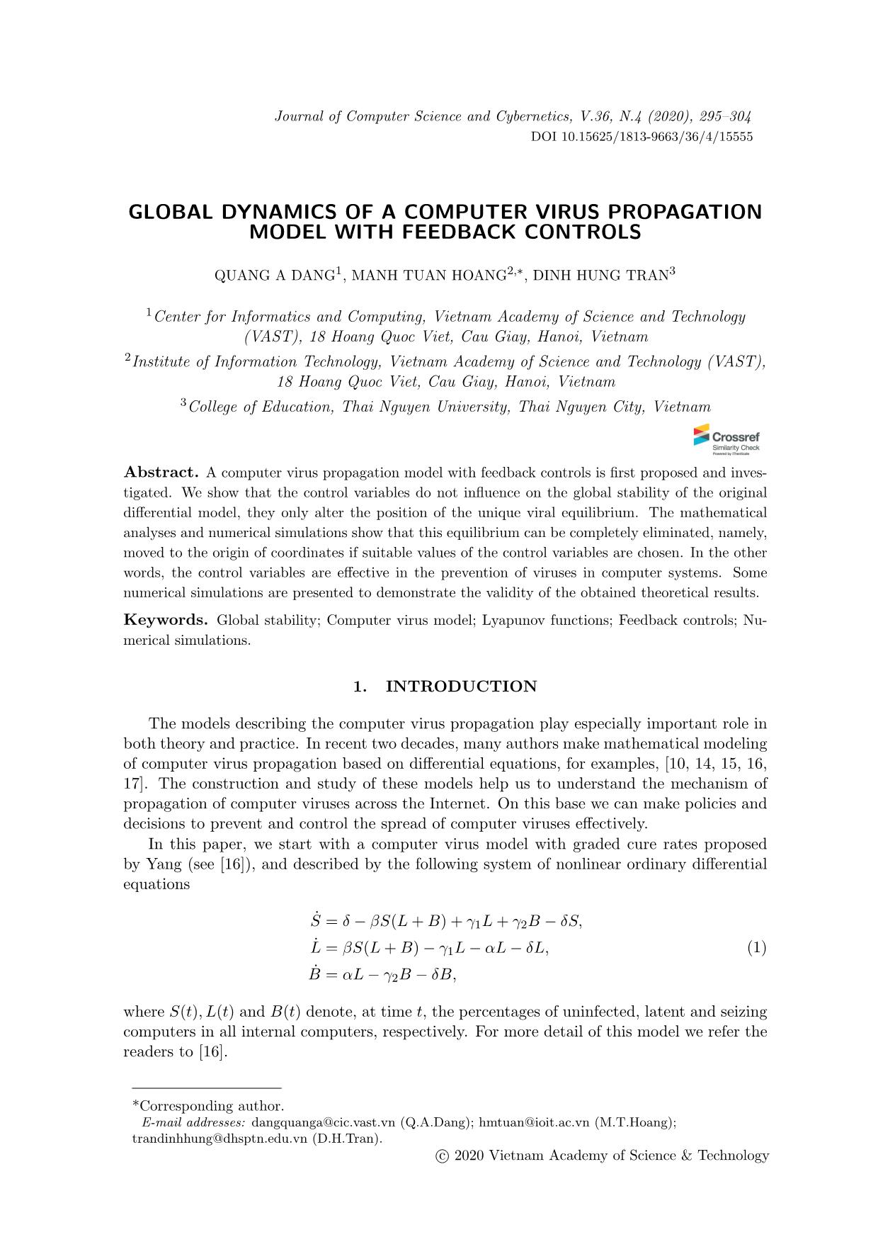
Abstract. A computer virus propagation model with feedback controls is first proposed and inves-
tigated. We show that the control variables do not influence on the global stability of the original
differential model, they only alter the position of the unique viral equilibrium. The mathematical
analyses and numerical simulations show that this equilibrium can be completely eliminated, namely,
moved to the origin of coordinates if suitable values of the control variables are chosen. In the other
words, the control variables are effective in the prevention of viruses in computer systems. Some
numerical simulations are presented to demonstrate the validity of the obtained theoretical results.
Keywords. Global stability; Computer virus model; Lyapunov functions; Feedback controls; Nu-
merical simulations.
1. INTRODUCTION
The models describing the computer virus propagation play especially important role in
both theory and practice. In recent two decades, many authors make mathematical modeling
of computer virus propagation based on differential equations, for examples, [10, 14, 15, 16,
17]. The construction and study of these models help us to understand the mechanism of
propagation of computer viruses across the Internet. On this base we can make policies and
decisions to prevent and control the spread of computer viruses effectively.
In this paper, we start with a computer virus model with graded cure rates proposed
by Yang (see [16]), and described by the following system of nonlinear ordinary differential
equations
S˙ = δ − βS(L+B) + γ1L+ γ2B − δS,
L˙ = βS(L+B)− γ1L− αL− δL,
B˙ = αL− γ2B − δB,
(1)
where S(t), L(t) and B(t) denote, at time t, the percentages of uninfected, latent and seizing
computers in all internal computers, respectively. For more detail of this model we refer the
readers to [16].
*Corresponding author.
E-mail addresses: dangquanga@cic.vast.vn (Q.A.Dang); hmtuan@ioit.ac.vn (M.T.Hoang);
trandinhhung@dhsptn.edu.vn (D.H.Tran).
c© 2020 Vietnam Academy of Science & Technology
296 QUANG A DANG, et al.
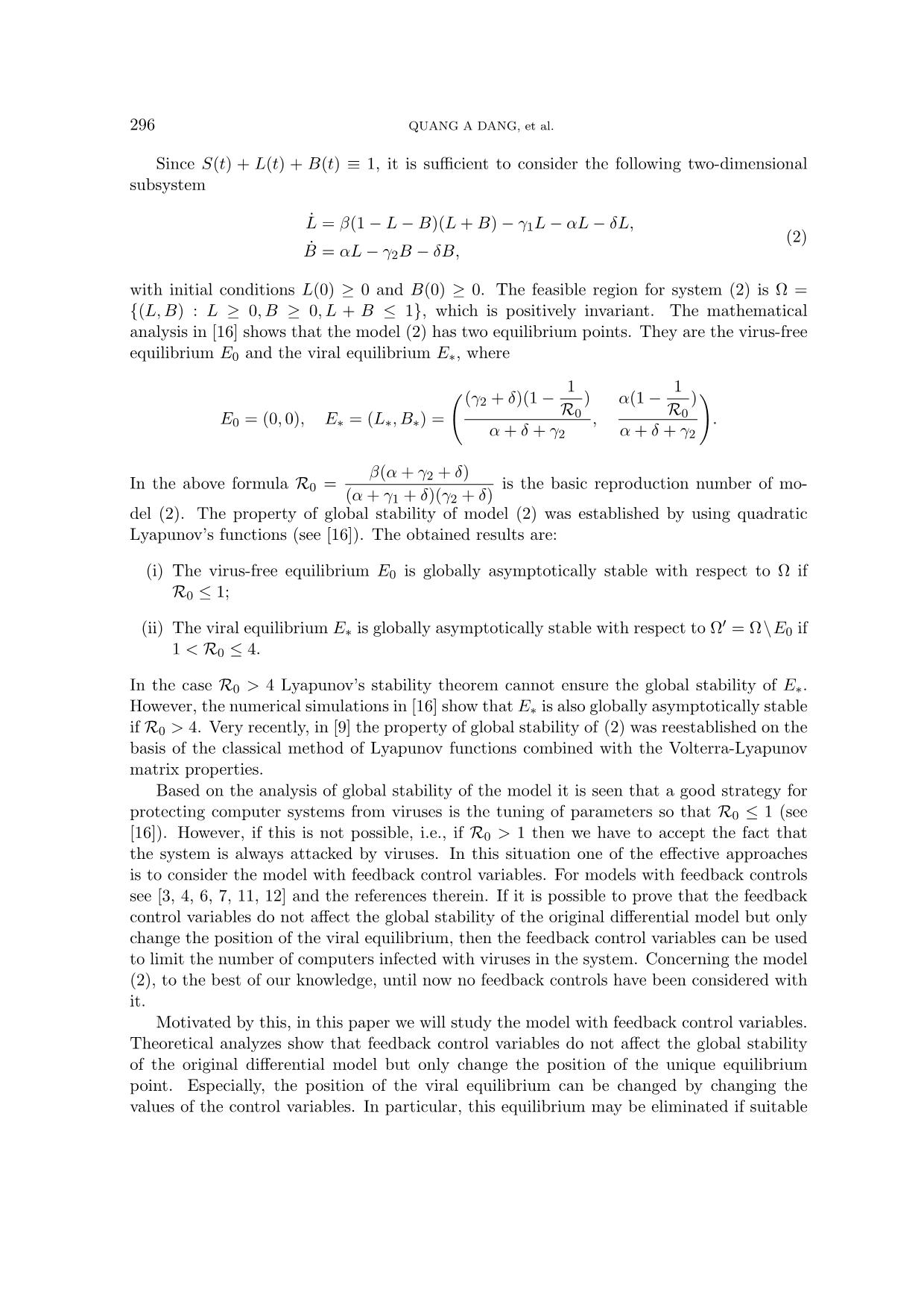
Since S(t) + L(t) + B(t) ≡ 1, it is sufficient to consider the following two-dimensional
subsystem
L˙ = β(1− L−B)(L+B)− γ1L− αL− δL,
B˙ = αL− γ2B − δB,
(2)
with initial conditions L(0) ≥ 0 and B(0) ≥ 0. The feasible region for system (2) is Ω =
{(L,B) : L ≥ 0, B ≥ 0, L + B ≤ 1}, which is positively invariant. The mathematical
analysis in [16] shows that the model (2) has two equilibrium points. They are the virus-free
equilibrium E0 and the viral equilibrium E∗, where
E0 = (0, 0), E∗ = (L∗, B∗) =
((γ2 + δ)(1− 1R0 )
α+ δ + γ2
,
α(1− 1R0 )
α+ δ + γ2
)
.
In the above formula R0 = β(α+ γ2 + δ)
(α+ γ1 + δ)(γ2 + δ)
is the basic reproduction number of mo-
del (2). The property of global stability of model (2) was established by using quadratic
Lyapunov’s functions (see [16]). The obtained results are:
(i) The virus-free equilibrium E0 is globally asymptotically stable with respect to Ω if
R0 ≤ 1;
(ii) The viral equilibrium E∗ is globally asymptotically stable with respect to Ω′ = Ω\E0 if
1 < R0 ≤ 4.
In the case R0 > 4 Lyapunov’s stability theorem cannot ensure the global stability of E∗.
However, the numerical simulations in [16] show that E∗ is also globally asymptotically stable
if R0 > 4. Very recently, in [9] the property of global stability of (2) was reestablished on the
basis of the classical method of Lyapunov functions combined with the Volterra-Lyapunov
matrix properties.
Based on the analysis of global stability of the model it is seen that a good strategy for
protecting computer systems from viruses is the tuning of parameters so that R0 ≤ 1 (see
[16]). However, if this is not possible, i.e., if R0 > 1 then we have to accept the fact that
the system is always attacked by viruses. In this situation one of the effective approaches
is to consider the model with feedback control variables. For models with feedback controls
see [3, 4, 6, 7, 11, 12] and the references therein. If it is possible to prove that the feedback
control variables do not affect the global stability of the original differential model but only
change the position of the viral equilibrium, then the feedback control variables can be used
to limit the number of computers infected with viruses in the system. Concerning the model
(2), to the best of our knowledge, until now no feedback controls have been considered with
it.
Motivated by this, in this paper we will study the model with feedback control variables.
Theoretical analyzes show that feedback control variables do not affect the global stability
of the original differential model but only change the position of the unique equilibrium
point. Especially, the position of the viral equilibrium can be changed by changing the
values of the control variables. In particular, this equilibrium may be eliminated if suitable
A COMPUTER VIRUS PROPAGATION MODEL 297
control variables are chosen. This result plays an important role in constructing strategies
for protection of computer systems.
To analyze the global stability of the proposed model, we use an appropriate Lyapunov for
investigating the global stability of the virus-free equilibrium. Meanwhile, in the context that
the proposed model consists of many equations and contains many parameters, the analysis
of stability of the positive equilibri ... s fact completely agrees with the related results of ordinary differential models in
ecology and epidemiology, namely, for the majority of models in these fields, if the positive
equilibrium points exist then they are globally asymptotically stable, i.e,. the models achieve
the robust development (see [1, 2]).
The paper is organized as follows. In Section 2, a model with feedback controls is pro-
posed. The global stability of the model is investigated in Section 3. Numerical simulations
are presented in Section 4. Finally, some conclusions are given in Section 5.
2. THE MODEL WITH FEEDBACK CONTROLS
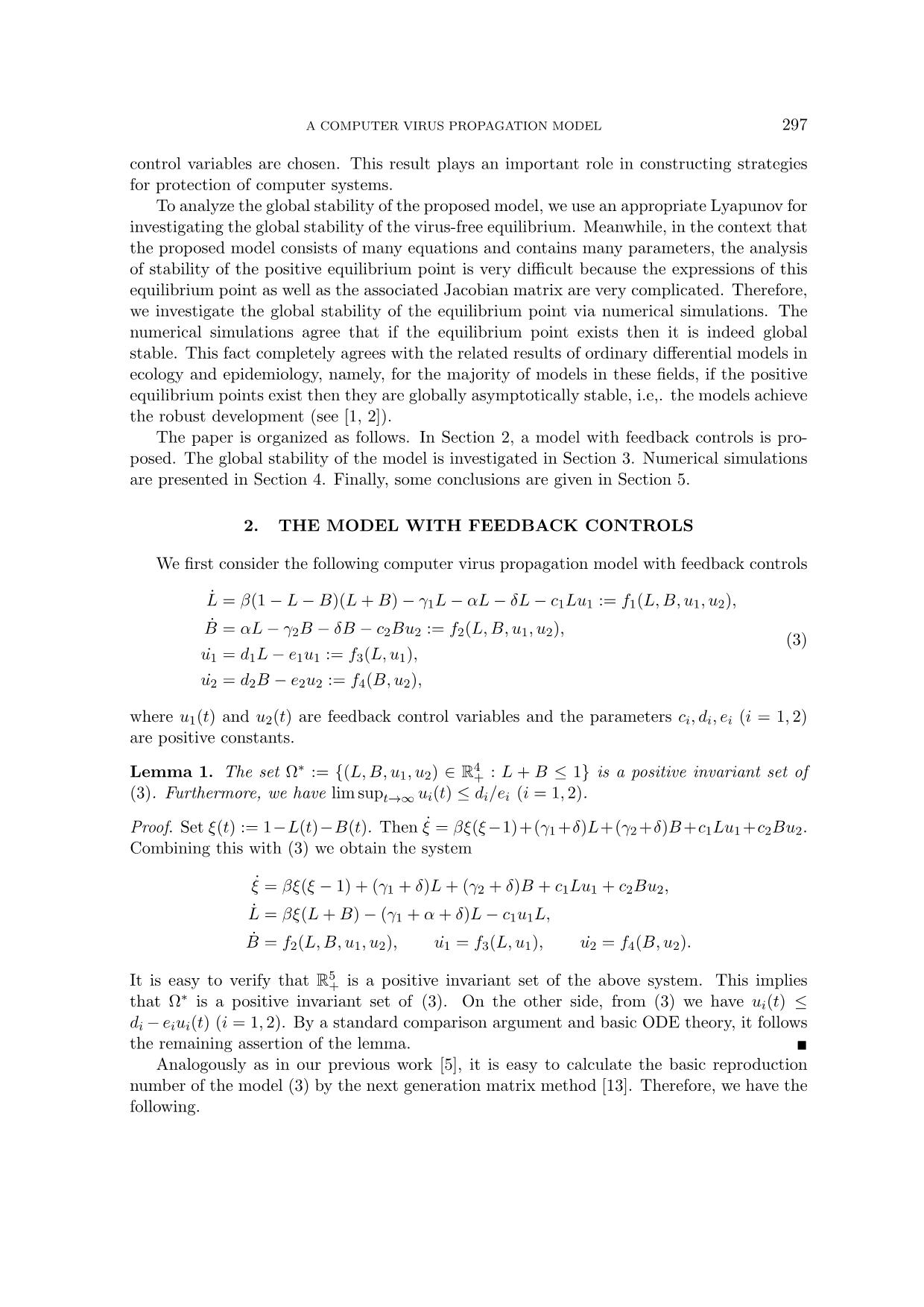
We first consider the following computer virus propagation model with feedback controls
L˙ = β(1− L−B)(L+B)− γ1L− αL− δL− c1Lu1 := f1(L,B, u1, u2),
B˙ = αL− γ2B − δB − c2Bu2 := f2(L,B, u1, u2),
u˙1 = d1L− e1u1 := f3(L, u1),
u˙2 = d2B − e2u2 := f4(B, u2),
(3)
where u1(t) and u2(t) are feedback control variables and the parameters ci, di, ei (i = 1, 2)
are positive constants.
Lemma 1. The set Ω∗ := {(L,B, u1, u2) ∈ R4+ : L + B ≤ 1} is a positive invariant set of
(3). Furthermore, we have lim supt→∞ ui(t) ≤ di/ei (i = 1, 2).
Proof. Set ξ(t) := 1−L(t)−B(t). Then ξ˙ = βξ(ξ−1)+(γ1+δ)L+(γ2+δ)B+c1Lu1+c2Bu2.
Combining this with (3) we obtain the system
ξ˙ = βξ(ξ − 1) + (γ1 + δ)L+ (γ2 + δ)B + c1Lu1 + c2Bu2,
L˙ = βξ(L+B)− (γ1 + α+ δ)L− c1u1L,
B˙ = f2(L,B, u1, u2), u˙1 = f3(L, u1), u˙2 = f4(B, u2).
It is easy to verify that R5+ is a positive invariant set of the above system. This implies
that Ω∗ is a positive invariant set of (3). On the other side, from (3) we have ui(t) ≤
di− eiui(t) (i = 1, 2). By a standard comparison argument and basic ODE theory, it follows
the remaining assertion of the lemma. 
Analogously as in our previous work [5], it is easy to calculate the basic reproduction
number of the model (3) by the next generation matrix method [13]. Therefore, we have the
following.
298 QUANG A DANG, et al.
Lemma 2. The number
R∗0 =
β(α+ γ2 + δ)
(α+ γ1 + δ)(γ2 + δ)
is the basic reproduction number of model (3).
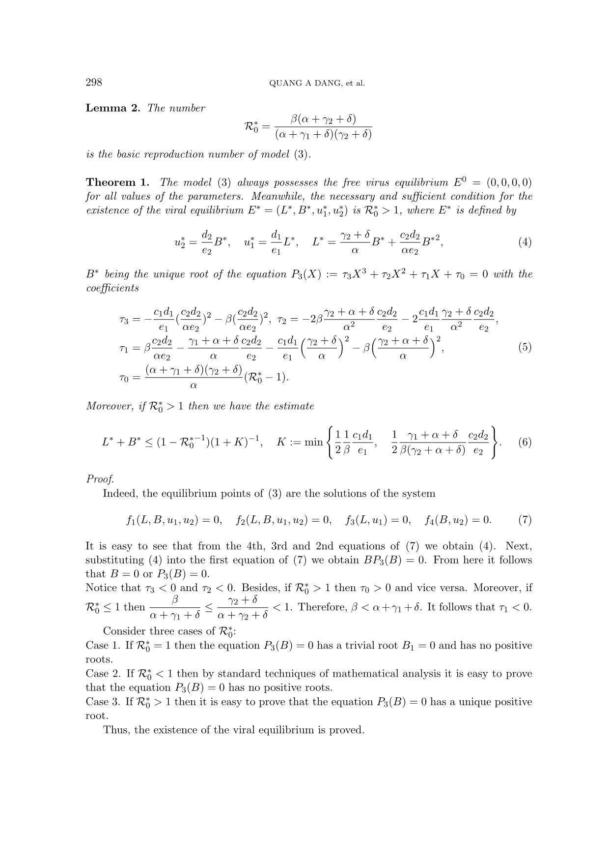
Theorem 1. The model (3) always possesses the free virus equilibrium E0 = (0, 0, 0, 0)
for all values of the parameters. Meanwhile, the necessary and sufficient condition for the
existence of the viral equilibrium E∗ = (L∗, B∗, u∗1, u∗2) is R∗0 > 1, where E∗ is defined by
u∗2 =
d2
e2
B∗, u∗1 =
d1
e1
L∗, L∗ =
γ2 + δ
α
B∗ +
c2d2
αe2
B∗2, (4)
B∗ being the unique root of the equation P3(X) := τ3X3 + τ2X2 + τ1X + τ0 = 0 with the
coefficients
τ3 = −c1d1
e1
(
c2d2
αe2
)2 − β(c2d2
αe2
)2, τ2 = −2βγ2 + α+ δ
α2
c2d2
e2
− 2c1d1
e1
γ2 + δ
α2
c2d2
e2
,
τ1 = β
c2d2
αe2
− γ1 + α+ δ
α
c2d2
e2
− c1d1
e1
(γ2 + δ
α
)2 − β(γ2 + α+ δ
α
)2
,
τ0 =
(α+ γ1 + δ)(γ2 + δ)
α
(R∗0 − 1).
(5)
Moreover, if R∗0 > 1 then we have the estimate
L∗ +B∗ ≤ (1−R∗0−1)(1 +K)−1, K := min
{
1
2
1
β
c1d1
e1
,
1
2
γ1 + α+ δ
β(γ2 + α+ δ)
c2d2
e2
}
. (6)
Proof.
Indeed, the equilibrium points of (3) are the solutions of the system
f1(L,B, u1, u2) = 0, f2(L,B, u1, u2) = 0, f3(L, u1) = 0, f4(B, u2) = 0. (7)
It is easy to see that from the 4th, 3rd and 2nd equations of (7) we obtain (4). Next,
substituting (4) into the first equation of (7) we obtain BP3(B) = 0. From here it follows
that B = 0 or P3(B) = 0.
Notice that τ3 1 then τ0 > 0 and vice versa. Moreover, if
R∗0 ≤ 1 then
β
α+ γ1 + δ
≤ γ2 + δ
α+ γ2 + δ
< 1. Therefore, β < α+γ1 + δ. It follows that τ1 < 0.
Consider three cases of R∗0:
Case 1. If R∗0 = 1 then the equation P3(B) = 0 has a trivial root B1 = 0 and has no positive
roots.
Case 2. If R∗0 < 1 then by standard techniques of mathematical analysis it is easy to prove
that the equation P3(B) = 0 has no positive roots.
Case 3. If R∗0 > 1 then it is easy to prove that the equation P3(B) = 0 has a unique positive
root.
Thus, the existence of the viral equilibrium is proved.
A COMPUTER VIRUS PROPAGATION MODEL 299
Next, consecutively multiplying the first and the second equations of (7) by γ2 + α + δ
and γ1 + α+ δ respectively, and adding side-by-side of the resulting equations we obtain
− β(γ2 + α+ δ)(L∗ +B∗)2 + (γ2 + δ)(γ1 + α+ δ)(R∗0 − 1)(L∗ +B∗)
− (γ2 + α+ δ)c1u∗1L∗ − (γ1 + α+ δ)c2u∗2B∗ = 0.
It follows that
L∗ +B∗ = (1−R∗0−1)−
[
1
β
c1u
∗
1L
∗ +
γ1 + α+ δ
β(γ2 + α+ δ)
c2u
∗
2B
∗
]
1
L∗ +B∗
.
Taking into account u∗1 =
d1L
∗
e1
, u∗2 =
d2B
∗
e2
and using the simple inequality 2(L2 +B2) ≥
(L+B)2 we obtain
1
β
c1u
∗
1L
∗ +
γ1 + α+ δ
β(γ2 + α+ δ)
c2u
∗
2B
∗ =
1
β
c1d1
e1
L∗2 +
γ1 + α+ δ
β(γ2 + α+ δ)
c2d2
e2
B∗2 ≥ K(L∗ +B∗)2.
Therefore,
L∗ +B∗ ≤ (1−R∗0−1)−K(L∗ +B∗).
From here it follows the inequality (6) to be proved. 
Remark.
Suppose it is proved that if the viral equilibrium exists (R∗0 > 1) then it is globally stable
(this result will be established in the next section). Then, we desire L∗ +B∗ to be as small
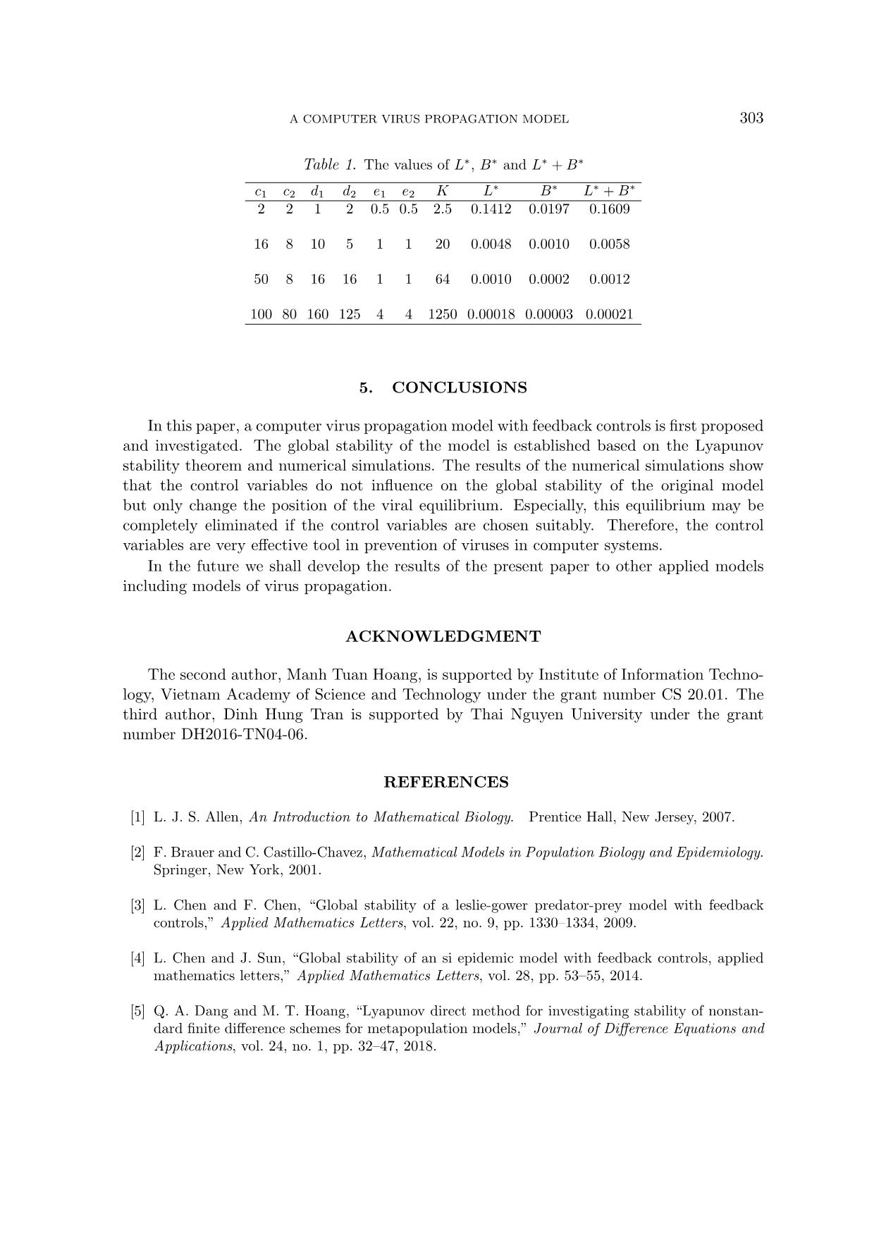
as possible. The estimate (6) shows that it is possible to make L∗ + B∗ arbitrarily small
by making K sufficiently large. This may be achieved because K depends on the control
variables (see Table 1 in Section 4.) Particularly, when K → ∞ then E∗ moves to the
origin, i.e., the viral equilibrium vanishes. In that time, for the model (2) we always have
L∗+B∗ = 1−R−10 (see [16]). This fact indirectly confirms the important role of the control
variables.
3. GLOBAL STABILITY OF THE MODEL WITH FEEDBACK
CONTROLS
In this section, we will establish the global stability property of the model (3).
3.1. Global stability of the equilibrium E0
The following theorem is of the global stability of E0 established with the use of a linear
Lyapunov function.
Theorem 2. The equilibrium point E0 is globally asymptotically stable of (3) in Ω∗ if
R∗0 ≤ 1.
300 QUANG A DANG, et al.
Proof.
We define the Lyapunov function V : Ω∗ → R+ by
V (L,B) = (α+ γ2 + δ)L+ (α+ γ1 + δ)B +
1
2
α+ γ2 + δ
d1
c1u
2
1 +
1
2
α+ γ1 + δ
d2
c2u
2
2.
The time derivative of the function V (L,B) along the trajectories of system (3) is
dV
dt
= [β(α+ γ2 + δ)− (γ2 + δ)(α+ γ1 + δ)]B + [β(α+ γ2 + δ)− (γ2 + δ)(α+ γ1 + δ)]L
− β(α+ γ2 + δ)(L+B)2 − α+ γ2 + δ
d1
e1c1u
2
1 −
α+ γ1 + δ
d2
e2c2u
2
2
≤ [β(α+ γ2 + δ)− (γ2 + δ)(α+ γ1 + δ)]B + [β(α+ γ2 + δ)− (γ2 + δ)(α+ γ1 + δ)]L
= (γ2 + δ)(α+ γ1 + δ)(R∗0 − 1)(L+B).
Obviously, dV /dt < 0 strictly for all (L,B) ∈ Ω∗ except for the equilibrium E0, where
dV /dt = 0. Hence, the function V satisfies Lyapunov’s asymptotic stability theorem [8], and
the equilibrium point E0 of system (3) is globally stable. 
3.2. Numerical simulations for investigating global stability of the positive equi-
librium point
In this subsection, some numerical simulations are performed to investigate the global
stability of the positive equilibrium point E∗. For this purpose, we consider model (3) with
the parameters
α = 0.1, β = 0.8, δ = 0.2, γ1 = 0.1, γ2 = 0.2.
In this case, we have R∗0 = 2.5 > 1. We select the control variables as follows
c1 = 1, c2 = 2, d1 = 1, d2 = 1.25, e1 = 2, e2 = 5.
Consequently, the unique positive equilibrium point is given by
E∗ = (0.3413, 0.0778, 0.1707, 0.0194).
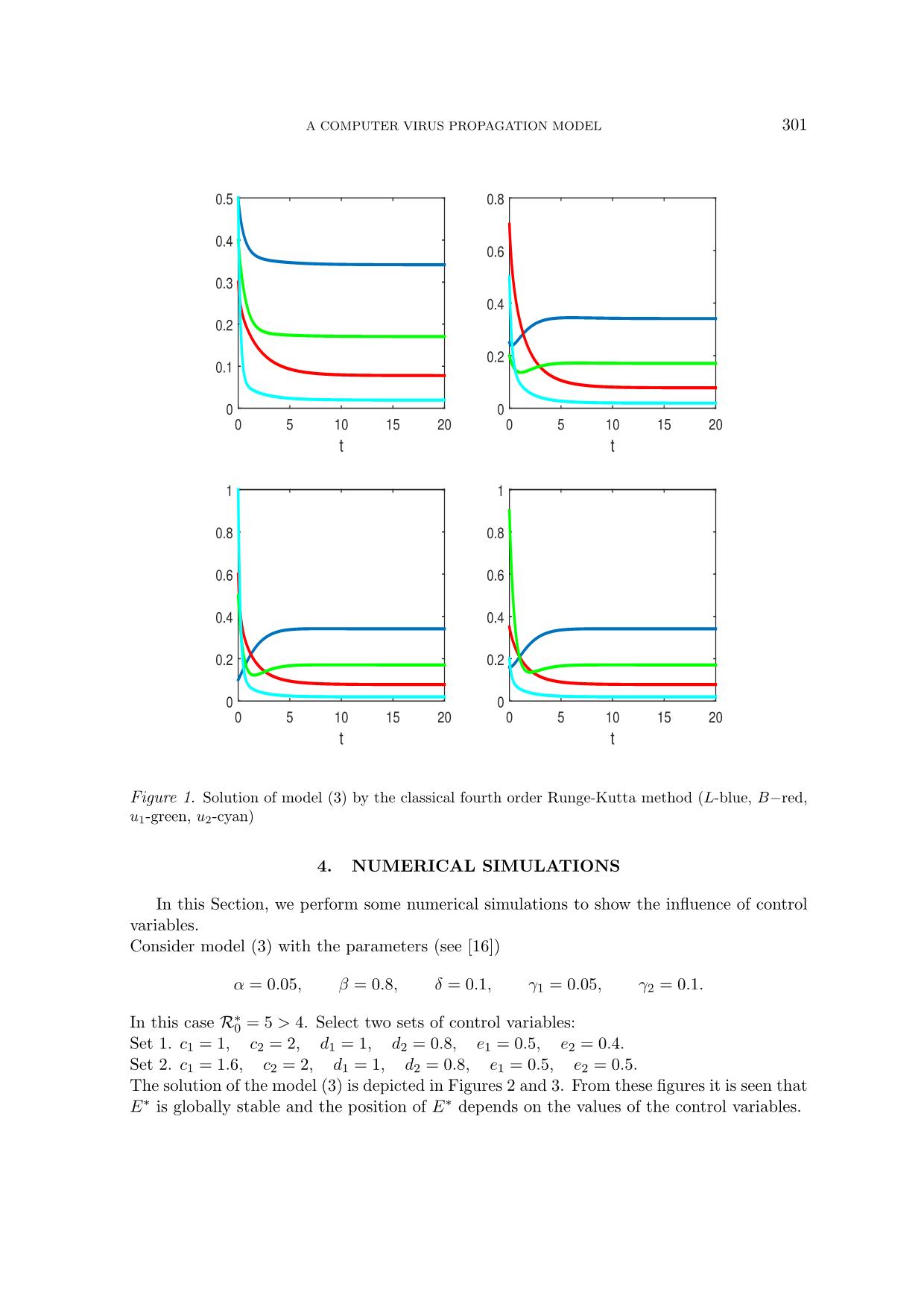
The solution of the model (3) with several initial values are depicted in Figure 1. From this
figure it is seen that E∗ is globally stable. It should be emphasized that all other numerical
simulations, including those in Section 4, give similar results. This means the global stability
of E∗ is observed.
A COMPUTER VIRUS PROPAGATION MODEL 301
t
0 5 10 15 20
0
0.1
0.2
0.3
0.4
0.5
t
0 5 10 15 20
0
0.2
0.4
0.6
0.8
t
0 5 10 15 20
0
0.2
0.4
0.6
0.8
1
t
0 5 10 15 20
0
0.2
0.4
0.6
0.8
1
Figure 1. Solution of model (3) by the classical fourth order Runge-Kutta method (L-blue, B−red,
u1-green, u2-cyan)
4. NUMERICAL SIMULATIONS
In this Section, we perform some numerical simulations to show the influence of control
variables.
Consider model (3) with the parameters (see [16])
α = 0.05, β = 0.8, δ = 0.1, γ1 = 0.05, γ2 = 0.1.
In this case R∗0 = 5 > 4. Select two sets of control variables:
Set 1. c1 = 1, c2 = 2, d1 = 1, d2 = 0.8, e1 = 0.5, e2 = 0.4.
Set 2. c1 = 1.6, c2 = 2, d1 = 1, d2 = 0.8, e1 = 0.5, e2 = 0.5.
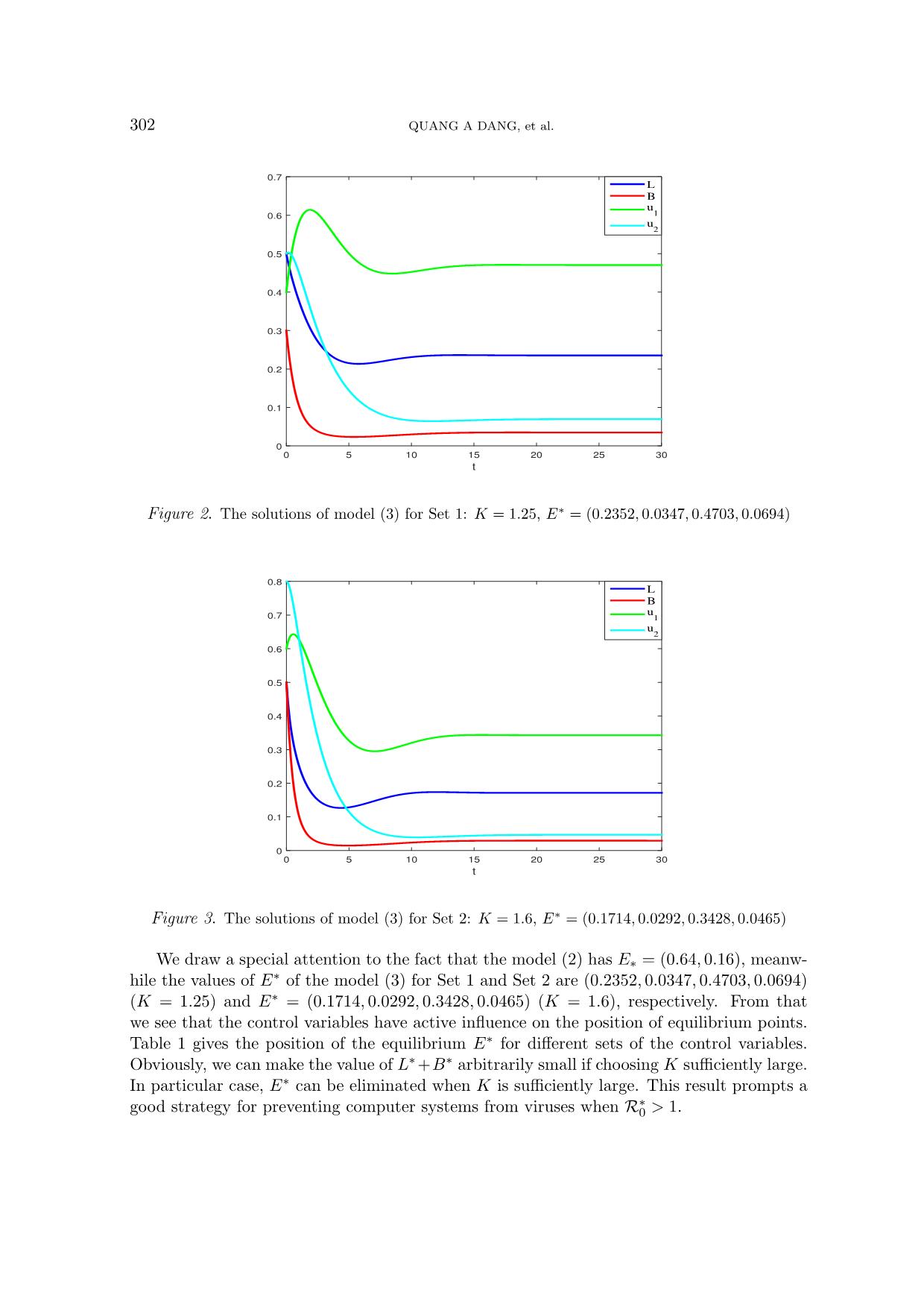
The solution of the model (3) is depicted in Figures 2 and 3. From these figures it is seen that
E∗ is globally stable and the position of E∗ depends on the values of the control variables.
302 QUANG A DANG, et al.
t
0 5 10 15 20 25 30
0
0.1
0.2
0.3
0.4
0.5
0.6
0.7
L
B
u1
u2
Figure 2. The solutions of model (3) for Set 1: K = 1.25, E∗ = (0.2352, 0.0347, 0.4703, 0.0694)
t
0 5 10 15 20 25 30
0
0.1
0.2
0.3
0.4
0.5
0.6
0.7
0.8
L
B
u1
u2
Figure 3. The solutions of model (3) for Set 2: K = 1.6, E∗ = (0.1714, 0.0292, 0.3428, 0.0465)
We draw a special attention to the fact that the model (2) has E∗ = (0.64, 0.16), meanw-
hile the values of E∗ of the model (3) for Set 1 and Set 2 are (0.2352, 0.0347, 0.4703, 0.0694)
(K = 1.25) and E∗ = (0.1714, 0.0292, 0.3428, 0.0465) (K = 1.6), respectively. From that
we see that the control variables have active influence on the position of equilibrium points.
Table 1 gives the position of the equilibrium E∗ for different sets of the control variables.
Obviously, we can make the value of L∗+B∗ arbitrarily small if choosing K sufficiently large.
In particular case, E∗ can be eliminated when K is sufficiently large. This result prompts a
good strategy for preventing computer systems from viruses when R∗0 > 1.
A COMPUTER VIRUS PROPAGATION MODEL 303
Table 1. The values of L∗, B∗ and L∗ +B∗
c1 c2 d1 d2 e1 e2 K L
∗ B∗ L∗ +B∗
2 2 1 2 0.5 0.5 2.5 0.1412 0.0197 0.1609
16 8 10 5 1 1 20 0.0048 0.0010 0.0058
50 8 16 16 1 1 64 0.0010 0.0002 0.0012
100 80 160 125 4 4 1250 0.00018 0.00003 0.00021
5. CONCLUSIONS
In this paper, a computer virus propagation model with feedback controls is first proposed
and investigated. The global stability of the model is established based on the Lyapunov
stability theorem and numerical simulations. The results of the numerical simulations show
that the control variables do not influence on the global stability of the original model
but only change the position of the viral equilibrium. Especially, this equilibrium may be
completely eliminated if the control variables are chosen suitably. Therefore, the control
variables are very effective tool in prevention of viruses in computer systems.
In the future we shall develop the results of the present paper to other applied models
including models of virus propagation.
ACKNOWLEDGMENT
The second author, Manh Tuan Hoang, is supported by Institute of Information Techno-
logy, Vietnam Academy of Science and Technology under the grant number CS 20.01. The
third author, Dinh Hung Tran is supported by Thai Nguyen University under the grant
number DH2016-TN04-06.
REFERENCES
[1] L. J. S. Allen, An Introduction to Mathematical Biology. Prentice Hall, New Jersey, 2007.
[2] F. Brauer and C. Castillo-Chavez, Mathematical Models in Population Biology and Epidemiology.
Springer, New York, 2001.
[3] L. Chen and F. Chen, “Global stability of a leslie-gower predator-prey model with feedback
controls,” Applied Mathematics Letters, vol. 22, no. 9, pp. 1330–1334, 2009.
[4] L. Chen and J. Sun, “Global stability of an si epidemic model with feedback controls, applied
mathematics letters,” Applied Mathematics Letters, vol. 28, pp. 53–55, 2014.
[5] Q. A. Dang and M. T. Hoang, “Lyapunov direct method for investigating stability of nonstan-
dard finite difference schemes for metapopulation models,” Journal of Difference Equations and
Applications, vol. 24, no. 1, pp. 32–47, 2018.
304 QUANG A DANG, et al.
[6] Q. A. Dang, M. T. Hoang, D. Y. Trejos, and J. C. Valverde, “Feedback control variables to
restrain the babesiosis disease,” Mathematical Methods in the Applied Sciences, vol. 42, pp.
7517–7527, 2019.
[7] H. L. Li, L. Zhang, Z. Teng, Y. L. Jiang, and A. Muhammadhaji, “Global stability of an si
epidemic model with feedback controls in a patchy environment,” Applied Mathematics and
Computation, vol. 321, pp. 372–384, 2018.
[8] A. M. Lyapunov, General Problem of the Stability of Motion. Taylor & Francis, London, 1992.
[9] M. R. Parsaei, R. Javidan, N. S. Kargar, and H. S. Nik, “On the global stability of an epidemic
model of computer viruses,” Theory in Biosciences, vol. 136, pp. 169–178, 2017.
[10] J. R. C. Piqueira and V. O. Araujo, “A modified epidemiological model for computer viruses,”
Applied Mathematics and Computation, vol. 213, pp. 355–360, 2009.
[11] Y. Shang, “Global stability of disease-free equilibria in a two-group si model with feedback
control,” Nonlinear Analysis: Modelling and Control, vol. 20, pp. 501–508, 2015.
[12] J. P. Tripathi and S. Abbas, “Global dynamics of autonomous and nonautonomous si epidemic
models with nonlinear incidence rate and feedback controls,” Nonlinear Dynamics, vol. 86, pp.
337–351, 2016.
[13] P. van den Driessche and J. Watmough, “Reproduction numbers and sub-threshold endemic
equilibria for compartmental models of disease transmission,” Mathematical Biosciences, vol.
180, pp. 29–48, 2002.
[14] L. Yang, X. Yang, L. Wen, and J. Liu, “A novel computer virus propagation model and its
dynamics,” International Journal of Computer Mathematics, vol. 89, pp. 2307–2314, 2012.
[15] L. X. Yang and X. Yang, “A new epidemic model of computer viruses,” Communications in
Nonlinear Science and Numerical Simulation, vol. 19, no. 9, pp. 1935–1944, 2014.
[16] L. X. Yang, X. Yang, Q. Zhu, and L. Wen, “A computer virus model with graded cure rates,”
Nonlinear Analysis: Real World Applications, vol. 14, pp. 414–422, 2013.
[17] X. Yang, B. K. Mishra, and Y. Liu, “Computer virus: theory, model, and methods,” Discrete
Dynamics in Nature and Society, pp. 473–508, 2012.
Received on September 30, 2020
Revised on October 21, 2020